Error function

Original article: w:Error function

Not to be confused with Loss function.

Error function
Plot of the error function
General information
General definition	$\operatorname {erf} z={\frac {2}{\sqrt {\pi }}}\int _{0}^{z}e^{-t^{2}}\,\mathrm {d} t$
Fields of application	Probability, thermodynamics
Domain, Codomain and Image
Domain	$\mathbb {C}$
Image	$\left(-1,1\right)$
Basic features
Parity	Odd
Specific features
Root	0
Derivative	${\frac {\mathrm {d} }{\mathrm {d} z}}\operatorname {erf} z={\frac {2}{\sqrt {\pi }}}e^{-z^{2}}$
Antiderivative	$\int \operatorname {erf} z\,dz=z\operatorname {erf} z+{\frac {e^{-z^{2}}}{\sqrt {\pi }}}+C$
Series definition
Taylor series	$\operatorname {erf} z={\frac {2}{\sqrt {\pi }}}\sum _{n=0}^{\infty }{\frac {z}{2n+1}}\prod _{k=1}^{n}{\frac {-z^{2}}{k}}$

수학(mathematics)에서, 오차 함수(error function)는, 역시 가우스 오차 함수(Gauss error function)라고 불리며, 종종 erf로 표시되며, 다음과 같이 정의된 복소 변수의 복소 함수입니다:

$\operatorname {erf} z={\frac {2}{\sqrt {\pi }}}\int _{0}^{z}e^{-t^{2}}\,\mathrm {d} t.$

이 적분은 종종 확률(probability), 통계(statistics), 및 부분 미분 방정식(partial differential equation)에서 발생하는 특수(special) (비-기본(elementary)) 시그모이드(sigmoid) 함수입니다. 많은 이들 응용에서, 그 함수 인수는 실수입니다. 만약 함수 인수가 실수이면, 함수 값은 역시 실수입니다.

통계에서, x의 비-음의 값에 대해, 오차 함수는 다음 해석을 가집니다: 평균(mean) 0과 표준 편차(standard deviation) ${\frac {1}{\sqrt {2}}}$를 갖는 정규적으로 분포된(normally distributed) 확률 변수(random variable) Y에 대해, erf x는 Y가 범위 [−x, x]에 떨어지는 확률입니다.

두 개의 밀접하게 관련된 함수는 다음과 같이 정의된 여 오차 함수(complementary error function, erfc)입니다:

$\operatorname {erfc} z=1-\operatorname {erf} z,$

그리고 다음과 같이 정의되는 허수 오차 함수(imaginary error function, erfi)입니다:

$\operatorname {erfi} z=-i\operatorname {erf} iz,$

여기서 i는 허수 단위(imaginary unit)입니다.

Name

"오차 함수"라는 이름과 그 약어 erf는 "the theory of Probability, and notably the theory of Errors"과의 관련 때문에 1871년 J. W. L. Glaisher에 의해 제안되었습니다. 오차 함수 여는 글레이셔에 의해 같은 해 별도의 간행물에서도 논의되었습니다. 그 밀도(density)가 다음에 의해 주어진 오차의 "편의의 법칙"에 대해

$f(x)=\left({\frac {c}{\pi }}\right)^{\frac {1}{2}}e^{-cx^{2}}$

(정규 분포(normal distribution)), 글레이셔는 p와 q 사이에 놓는 오차의 확률을 다음과 같이 계산합니다:

$\left({\frac {c}{\pi }}\right)^{\frac {1}{2}}\int _{p}^{q}e^{-cx^{2}}\,\mathrm {d} x={\tfrac {1}{2}}\left(\operatorname {erf} \left(q{\sqrt {c}}\right)-\operatorname {erf} \left(p{\sqrt {c}}\right)\right).$

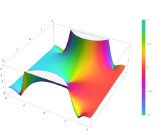
Plot of the error function Erf(z) in the complex plane from -2-2i to 2+2i with colors created with Mathematica 13.1 function ComplexPlot3D

Applications

일련의 측정의 결과가 표준 편차(standard deviation) σ와 기댓값(expected value) 0을 갖는 정규 분포(normal distribution)에 의해 설명될 때, erf (a/σ √2)는 단일 측정의 오차가 양수 a에 대해 −a와 +a 사이에 놓을 확률입니다. 이것은, 예를 들어, 이것은 디지털 통신 시스템의 비트 오류율(bit error rate)을 결정하는 데 유용합니다.

오차 함수와 여 오차 함수는, 예를 들어, 경계 조건(boundary conditions)이 헤비사이드 계단 함수(Heaviside step function)에 의해 제공될 때 열 방정식(heat equation)의 해에서 발생합니다.

오차 함수와 그 근사는 높은 확률(with high probability) 또는 낮은 확률로 유지되는 결과를 추정하기 위해 사용될 수 있습니다. 확률 변수 X ~ Norm[μ,σ] (평균 μ와 표준 편차 σ를 갖는 정규 분포)와 상수 L < μ가 주어지면:

${\begin{aligned}\Pr[X\leq L]&={\frac {1}{2}}+{\frac {1}{2}}\operatorname {erf} {\frac {L-\mu }{{\sqrt {2}}\sigma }}\\&\approx A\exp \left(-B\left({\frac {L-\mu }{\sigma }}\right)^{2}\right)\end{aligned}}$

여기서 A와 B는 특정 숫자 상수입니다. 만약 L이 평균에서 충분하게 멀리 있으면, 구체적으로 μ − L ≥ σ√ln k이면, 다음과 같습니다:

$\Pr[X\leq L]\leq A\exp(-B\ln {k})={\frac {A}{k^{B}}}$

따라서 k → ∞일 때 확률은 0으로 갑니다.

X가 구간 [L_a, L_b]에 있을 확률은 다음과 같이 유도될 수 있습니다:

${\begin{aligned}\Pr[L_{a}\leq X\leq L_{b}]&=\int _{L_{a}}^{L_{b}}{\frac {1}{{\sqrt {2\pi }}\sigma }}\exp \left(-{\frac {(x-\mu )^{2}}{2\sigma ^{2}}}\right)\,\mathrm {d} x\\&={\frac {1}{2}}\left(\operatorname {erf} {\frac {L_{b}-\mu }{{\sqrt {2}}\sigma }}-\operatorname {erf} {\frac {L_{a}-\mu }{{\sqrt {2}}\sigma }}\right).\end{aligned}}$

Properties

Plots in the complex plane

Integrand exp(−z²)

erf z

속성 erf (−z) = −erf z는 오차 함수가 홀수 함수(odd function)임을 의미합니다. 이것은 피적분 e^−t2가 짝수 함수(even function)라는 사실에서 직접적으로 발생합니다 (원점에서 영인 짝수 함수의 역도함수는 홀수 함수이고 그 반대도 마찬가지입니다).

오차 함수는 실수를 실수로 취하는 전체 함수(entire function)이기 때문에, 임의의 복소수(complex number) z에 대해, 다음과 같습니다:

$\operatorname {erf} {\overline {z}}={\overline {\operatorname {erf} z}}$

여기서 z는 z의 복소 켤레(complex conjugate)입니다.

피적분 f = exp(−z²)과 f = erf z는 오른쪽 그림의 복소수 z-평면에 도메인 색칠(domain coloring)로 표시되어 있습니다.

+∞에서의 오차 함수는 정확히 1입니다 (가우스 적분(Gaussian integral)을 참조하십시오). 실수 축에서, erf z는 z → +∞에서 단위로 접근하고 z → −∞에서 −1에 접근합니다. 허수 축에서, 그것은 ±i∞로 가는 경향이 있습니다.

Taylor series

오차 함수는 전체 함수(entire function)입니다; 그것은 특이점을 가지지 않고 (무한대에서 제외) 그것의 테일러 전개(Taylor expansion)는 항상 수렴하지만, "[...] x > 1이면 잘못된 수렴에 대해" 유명하게 알려져 있습니다.

정의하는 적분은 기본 함수(elementary functions)의 측면에서 닫힌 형식(closed form)으로 평가될 수 없지만, 피적분(integrand) e^−z2를 그것의 매클로린 급수(Maclaurin series)로 전개하고 항-별로 적분함으로써, 오차 함수의 매클로린 급수를 다음과 같이 얻습니다:

${\begin{aligned}\operatorname {erf} z&={\frac {2}{\sqrt {\pi }}}\sum _{n=0}^{\infty }{\frac {(-1)^{n}z^{2n+1}}{n!(2n+1)}}\\[6pt]&={\frac {2}{\sqrt {\pi }}}\left(z-{\frac {z^{3}}{3}}+{\frac {z^{5}}{10}}-{\frac {z^{7}}{42}}+{\frac {z^{9}}{216}}-\cdots \right)\end{aligned}}$

이는 모든 각 복소수(complex number) z에 유지됩니다. 분모 항은 OEIS에서 수열 A007680입니다.

위 급수의 반복 계산을 위해, 다음 대안적인 공식이 유용할 수 있습니다:

${\begin{aligned}\operatorname {erf} z&={\frac {2}{\sqrt {\pi }}}\sum _{n=0}^{\infty }\left(z\prod _{k=1}^{n}{\frac {-(2k-1)z^{2}}{k(2k+1)}}\right)\\[6pt]&={\frac {2}{\sqrt {\pi }}}\sum _{n=0}^{\infty }{\frac {z}{2n+1}}\prod _{k=1}^{n}{\frac {-z^{2}}{k}}\end{aligned}}$

왜냐하면 −(2k − 1)z²/k(2k + 1)은 k번째 항을 (k + 1)번째 항으로 바꾸는 곱셈수를 나타내기 때문입니다 (z를 첫 번째 항으로 고려합니다).

허수 오차 함수는 다음과 같은 매우 유사한 매클로린 급수를 가집니다:

${\begin{aligned}\operatorname {erfi} z&={\frac {2}{\sqrt {\pi }}}\sum _{n=0}^{\infty }{\frac {z^{2n+1}}{n!(2n+1)}}\\[6pt]&={\frac {2}{\sqrt {\pi }}}\left(z+{\frac {z^{3}}{3}}+{\frac {z^{5}}{10}}+{\frac {z^{7}}{42}}+{\frac {z^{9}}{216}}+\cdots \right)\end{aligned}}$

이는 모든 각 복소수(complex number) z에 유지됩니다.

Derivative and integral

오차 함수의 도함수는 정의에서 바로 이어집니다:

${\frac {\mathrm {d} }{\mathrm {d} z}}\operatorname {erf} z={\frac {2}{\sqrt {\pi }}}e^{-z^{2}}.$

이로부터, 허수 오차 함수의 도함수도 즉각적입니다:

${\frac {d}{dz}}\operatorname {erfi} z={\frac {2}{\sqrt {\pi }}}e^{z^{2}}.$

부분에 의한 적분(integration by parts)으로 얻어질 수 있는 오차 함수의 역도함수(antiderivative)는 다음과 같습니다:

$z\operatorname {erf} z+{\frac {e^{-z^{2}}}{\sqrt {\pi }}}.$

허수 오차 함수의 역도함수는, 역시 부분에 의한 적분으로 얻어질 수 있으며, 다음과 같습니다:

$z\operatorname {erfi} z-{\frac {e^{z^{2}}}{\sqrt {\pi }}}.$

고차 도함수는 다음과 같이 지정됩니다:

$\operatorname {erf} ^{(k)}z={\frac {2(-1)^{k-1}}{\sqrt {\pi }}}{\mathit {H}}_{k-1}(z)e^{-z^{2}}={\frac {2}{\sqrt {\pi }}}{\frac {\mathrm {d} ^{k-1}}{\mathrm {d} z^{k-1}}}\left(e^{-z^{2}}\right),\qquad k=1,2,\dots$

여기서 H는 물리학자의 에르미트 다항식(Hermite polynomials)입니다.

Bürmann series

전개는, x의 모든 실수 값에 대해 테일러 전개보다 더 빠르게 수렴하며, 한스 하인리히 뷔르만(Hans Heinrich Bürmann)의 정리를 사용함으로써 얻습니다:

${\begin{aligned}\operatorname {erf} x&={\frac {2}{\sqrt {\pi }}}\operatorname {sgn} x\cdot {\sqrt {1-e^{-x^{2}}}}\left(1-{\frac {1}{12}}\left(1-e^{-x^{2}}\right)-{\frac {7}{480}}\left(1-e^{-x^{2}}\right)^{2}-{\frac {5}{896}}\left(1-e^{-x^{2}}\right)^{3}-{\frac {787}{276480}}\left(1-e^{-x^{2}}\right)^{4}-\cdots \right)\\[10pt]&={\frac {2}{\sqrt {\pi }}}\operatorname {sgn} x\cdot {\sqrt {1-e^{-x^{2}}}}\left({\frac {\sqrt {\pi }}{2}}+\sum _{k=1}^{\infty }c_{k}e^{-kx^{2}}\right).\end{aligned}}$

여기서 sgn은 부호 함수(sign function)입니다. 처음 두 계수만 유지하고 c₁ = 31/200와 c₂ = −341/8000을 선택함으로써, 결과 근사는 x = ±1.3796에서 가장 큰 상대 오차를 보이며, 그곳에서 오차는 0.0036127보다 작습니다:

$\operatorname {erf} x\approx {\frac {2}{\sqrt {\pi }}}\operatorname {sgn} x\cdot {\sqrt {1-e^{-x^{2}}}}\left({\frac {\sqrt {\pi }}{2}}+{\frac {31}{200}}e^{-x^{2}}-{\frac {341}{8000}}e^{-2x^{2}}\right).$

Inverse functions

Inverse error function

복소수 z가 주어지면, erf w = z를 만족시키는 고유한 복소수 w가 없으므로, 참 역 함수는 다중값이 됩니다. 어쨌든, −1 < x < 1에 대해, 다음을 만족시키는 erf⁻¹ x로 표시된 고유한 실수가 있습니다:

$\operatorname {erf} \left(\operatorname {erf} ^{-1}x\right)=x.$

역 오차 함수(inverse error function)는 보통 도메인 (−1,1)로 정의되고, 많은 컴퓨터 대수 시스템에서 이 도메인으로 제한됩니다. 어쨌든, 그것은 매클로린 급수를 사용하여 복소 평면의 디스크 |z| < 1로 확장될 수 있습니다:

$\operatorname {erf} ^{-1}z=\sum _{k=0}^{\infty }{\frac {c_{k}}{2k+1}}\left({\frac {\sqrt {\pi }}{2}}z\right)^{2k+1},$

여기서 c₀ = 1이고 다음과 같습니다:

${\begin{aligned}c_{k}&=\sum _{m=0}^{k-1}{\frac {c_{m}c_{k-1-m}}{(m+1)(2m+1)}}\\&=\left\{1,1,{\frac {7}{6}},{\frac {127}{90}},{\frac {4369}{2520}},{\frac {34807}{16200}},\ldots \right\}.\end{aligned}}$

따라서 우리는 다음과 같은 급수 전개를 가집니다 (공통 인수는 분자와 분모에서 취소됩니다):

$\operatorname {erf} ^{-1}z={\frac {\sqrt {\pi }}{2}}\left(z+{\frac {\pi }{12}}z^{3}+{\frac {7\pi ^{2}}{480}}z^{5}+{\frac {127\pi ^{3}}{40320}}z^{7}+{\frac {4369\pi ^{4}}{5806080}}z^{9}+{\frac {34807\pi ^{5}}{182476800}}z^{11}+\cdots \right).$

(취소 후, 분자/분모 분수는 OEIS에서 엔트리 OEIS: A092676/OEIS: A092677입니다. 취소 없이, 분자 항은 엔트리 OEIS: A002067에서 제공됩니다.) ±∞에서 오차 함수의 값은 ±1과 같습니다.

|z| < 1에 대해, 우리는 erf(erf⁻¹ z) = z를 가집니다.

역 여 오차 함수(inverse complementary error function)는 다음과 같이 정의됩니다:

$\operatorname {erfc} ^{-1}(1-z)=\operatorname {erf} ^{-1}z.$

실수 x에 대해, erfi(erfi⁻¹ x) = x를 만족시키는 고유한 실수 erfi⁻¹ x가 있습니다. 역 허수 오차 함수(inverse imaginary error function)는 erfi⁻¹ x로 정의됩니다.

임의의 실수 x에 대해, 뉴턴의 방법(Newton's method)은 erfi⁻¹ x를 계산하기 위해 사용될 수 있고, −1 ≤ x ≤ 1에 대해, 다음 매클로린 급수는 수렴합니다:

$\operatorname {erfi} ^{-1}z=\sum _{k=0}^{\infty }{\frac {(-1)^{k}c_{k}}{2k+1}}\left({\frac {\sqrt {\pi }}{2}}z\right)^{2k+1},$

여기서 c_k는 위에서 처럼 정의됩니다.

Asymptotic expansion

A useful asymptotic expansion of the complementary error function (and therefore also of the error function) for large real x is

${\begin{aligned}\operatorname {erfc} x&={\frac {e^{-x^{2}}}{x{\sqrt {\pi }}}}\left(1+\sum _{n=1}^{\infty }(-1)^{n}{\frac {1\cdot 3\cdot 5\cdots (2n-1)}{\left(2x^{2}\right)^{n}}}\right)\\[6pt]&={\frac {e^{-x^{2}}}{x{\sqrt {\pi }}}}\sum _{n=0}^{\infty }(-1)^{n}{\frac {(2n-1)!!}{\left(2x^{2}\right)^{n}}},\end{aligned}}$

where (2n − 1)!! is the double factorial of (2n − 1), which is the product of all odd numbers up to (2n − 1). This series diverges for every finite x, and its meaning as asymptotic expansion is that for any integer N ≥ 1 one has

$\operatorname {erfc} x={\frac {e^{-x^{2}}}{x{\sqrt {\pi }}}}\sum _{n=0}^{N-1}(-1)^{n}{\frac {(2n-1)!!}{\left(2x^{2}\right)^{n}}}+R_{N}(x)$

where the remainder, in Landau notation, is

$R_{N}(x)=O\left(x^{-(1+2N)}e^{-x^{2}}\right)$

as x → ∞.

Indeed, the exact value of the remainder is

$R_{N}(x):={\frac {(-1)^{N}}{\sqrt {\pi }}}2^{1-2N}{\frac {(2N)!}{N!}}\int _{x}^{\infty }t^{-2N}e^{-t^{2}}\,\mathrm {d} t,$

which follows easily by induction, writing

$e^{-t^{2}}=-(2t)^{-1}\left(e^{-t^{2}}\right)'$

and integrating by parts.

For large enough values of x, only the first few terms of this asymptotic expansion are needed to obtain a good approximation of erfc x (while for not too large values of x, the above Taylor expansion at 0 provides a very fast convergence).

Continued fraction expansion

A continued fraction expansion of the complementary error function is:

$\operatorname {erfc} z={\frac {z}{\sqrt {\pi }}}e^{-z^{2}}{\cfrac {1}{z^{2}+{\cfrac {a_{1}}{1+{\cfrac {a_{2}}{z^{2}+{\cfrac {a_{3}}{1+\dotsb }}}}}}}},\qquad a_{m}={\frac {m}{2}}.$

Integral of error function with Gaussian density function

$\int _{-\infty }^{\infty }\operatorname {erf} \left(ax+b\right){\frac {1}{\sqrt {2\pi \sigma ^{2}}}}\exp \left(-{\frac {(x-\mu )^{2}}{2\sigma ^{2}}}\right)\,\mathrm {d} x=\operatorname {erf} {\frac {a\mu +b}{\sqrt {1+2a^{2}\sigma ^{2}}}},\qquad a,b,\mu ,\sigma \in \mathbb {R}$

which appears related to Ng and Geller, formula 13 in section 4.3 with a change of variables.

Factorial series

The inverse factorial series:

${\begin{aligned}\operatorname {erfc} z&={\frac {e^{-z^{2}}}{{\sqrt {\pi }}\,z}}\sum _{n=0}^{\infty }{\frac {(-1)^{n}Q_{n}}{{(z^{2}+1)}^{\bar {n}}}}\\&={\frac {e^{-z^{2}}}{{\sqrt {\pi }}\,z}}\left(1-{\frac {1}{2}}{\frac {1}{(z^{2}+1)}}+{\frac {1}{4}}{\frac {1}{(z^{2}+1)(z^{2}+2)}}-\cdots \right)\end{aligned}}$

converges for Re(z²) > 0. Here

${\begin{aligned}Q_{n}&{\overset {\text{def}}{{}={}}}{\frac {1}{\Gamma \left({\frac {1}{2}}\right)}}\int _{0}^{\infty }\tau (\tau -1)\cdots (\tau -n+1)\tau ^{-{\frac {1}{2}}}e^{-\tau }\,d\tau \\&=\sum _{k=0}^{n}\left({\tfrac {1}{2}}\right)^{\bar {k}}s(n,k),\end{aligned}}$

zⁿ denotes the rising factorial, and s(n,k) denotes a signed Stirling number of the first kind. There also exists a representation by an infinite sum containing the double factorial:

$\operatorname {erf} z={\frac {2}{\sqrt {\pi }}}\sum _{n=0}^{\infty }{\frac {(-2)^{n}(2n-1)!!}{(2n+1)!}}z^{2n+1}$

Numerical approximations

Approximation with elementary functions

• Abramowitz and Stegun give several approximations of varying accuracy (equations 7.1.25–28). This allows one to choose the fastest approximation suitable for a given application. In order of increasing accuracy, they are:

  $\operatorname {erf} x\approx 1-{\frac {1}{\left(1+a_{1}x+a_{2}x^{2}+a_{3}x^{3}+a_{4}x^{4}\right)^{4}}},\qquad x\geq 0$

  (maximum error: 5×10⁻⁴)

  where a₁ = 0.278393, a₂ = 0.230389, a₃ = 0.000972, a₄ = 0.078108

  $\operatorname {erf} x\approx 1-\left(a_{1}t+a_{2}t^{2}+a_{3}t^{3}\right)e^{-x^{2}},\quad t={\frac {1}{1+px}},\qquad x\geq 0$

  (maximum error: 2.5×10⁻⁵)

  where p = 0.47047, a₁ = 0.3480242, a₂ = −0.0958798, a₃ = 0.7478556

  $$\operatorname {erf} x\approx 1-{\frac {1}{\left(1+a_{1}x+a_{2}x^{2}+\cdots +a_{6}x^{6}\right)^{16}}},\qquad x\geq 0$$ (maximum error: 3×10⁻⁷)

  where a₁ = 0.0705230784, a₂ = 0.0422820123, a₃ = 0.0092705272, a₄ = 0.0001520143, a₅ = 0.0002765672, a₆ = 0.0000430638

  $$\operatorname {erf} x\approx 1-\left(a_{1}t+a_{2}t^{2}+\cdots +a_{5}t^{5}\right)e^{-x^{2}},\quad t={\frac {1}{1+px}}$$ (maximum error: 1.5×10⁻⁷)

  where p = 0.3275911, a₁ = 0.254829592, a₂ = −0.284496736, a₃ = 1.421413741, a₄ = −1.453152027, a₅ = 1.061405429

  All of these approximations are valid for x ≥ 0. To use these approximations for negative x, use the fact that erf x is an odd function, so erf x = −erf(−x).
• Exponential bounds and a pure exponential approximation for the complementary error function are given by

  ${\begin{aligned}\operatorname {erfc} x&\leq {\tfrac {1}{2}}e^{-2x^{2}}+{\tfrac {1}{2}}e^{-x^{2}}\leq e^{-x^{2}},&\quad x&>0\\\operatorname {erfc} x&\approx {\tfrac {1}{6}}e^{-x^{2}}+{\tfrac {1}{2}}e^{-{\frac {4}{3}}x^{2}},&\quad x&>0.\end{aligned}}$

• The above have been generalized to sums of N exponentials with increasing accuracy in terms of N so that erfc x can be accurately approximated or bounded by 2Q̃(√2x), where

  ${\tilde {Q}}(x)=\sum _{n=1}^{N}a_{n}e^{-b_{n}x^{2}}.$

  In particular, there is a systematic methodology to solve the numerical coefficients {(a_n,b_n)}^N
  _{n = 1} that yield a minimax approximation or bound for the closely related Q-function: Q(x) ≈ Q̃(x), Q(x) ≤ Q̃(x), or Q(x) ≥ Q̃(x) for x ≥ 0. The coefficients {(a_n,b_n)}^N
  _{n = 1} for many variations of the exponential approximations and bounds up to N = 25 have been released to open access as a comprehensive dataset.
• A tight approximation of the complementary error function for x ∈ [0,∞) is given by Karagiannidis & Lioumpas (2007) who showed for the appropriate choice of parameters {A,B} that

  $\operatorname {erfc} x\approx {\frac {\left(1-e^{-Ax}\right)e^{-x^{2}}}{B{\sqrt {\pi }}x}}.$

  They determined {A,B} = {1.98,1.135}, which gave a good approximation for all x ≥ 0. Alternative coefficients are also available for tailoring accuracy for a specific application or transforming the expression into a tight bound.
• A single-term lower bound is

  $$\operatorname {erfc} x\geq {\sqrt {\frac {2e}{\pi }}}{\frac {\sqrt {\beta -1}}{\beta }}e^{-\beta x^{2}},\qquad x\geq 0,\quad \beta >1,$$

  where the parameter β can be picked to minimize error on the desired interval of approximation.
• Another approximation is given by Sergei Winitzki using his "global Padé approximations":

  $\operatorname {erf} x\approx \operatorname {sgn} x\cdot {\sqrt {1-\exp \left(-x^{2}{\frac {{\frac {4}{\pi }}+ax^{2}}{1+ax^{2}}}\right)}}$

  where

  $a={\frac {8(\pi -3)}{3\pi (4-\pi )}}\approx 0.140012.$

  This is designed to be very accurate in a neighborhood of 0 and a neighborhood of infinity, and the relative error is less than 0.00035 for all real x. Using the alternate value a ≈ 0.147 reduces the maximum relative error to about 0.00013.

  This approximation can be inverted to obtain an approximation for the inverse error function:

  $\operatorname {erf} ^{-1}x\approx \operatorname {sgn} x\cdot {\sqrt {{\sqrt {\left({\frac {2}{\pi a}}+{\frac {\ln \left(1-x^{2}\right)}{2}}\right)^{2}-{\frac {\ln \left(1-x^{2}\right)}{a}}}}-\left({\frac {2}{\pi a}}+{\frac {\ln \left(1-x^{2}\right)}{2}}\right)}}.$

• An approximation with a maximal error of 1.2×10⁻⁷ for any real argument is:

  $\operatorname {erf} x={\begin{cases}1-\tau &x\geq 0\\\tau -1&x<0\end{cases}}$

  with

  ${\begin{aligned}\tau &=t\cdot \exp \left(-x^{2}-1.26551223+1.00002368t+0.37409196t^{2}+0.09678418t^{3}-0.18628806t^{4}\right.\\&\left.\qquad \qquad \qquad +0.27886807t^{5}-1.13520398t^{6}+1.48851587t^{7}-0.82215223t^{8}+0.17087277t^{9}\right)\end{aligned}}$

  and

  $t={\frac {1}{1+{\frac {1}{2}}|x|}}.$

Table of values

Further information: Interval estimation, Coverage probability, and 68–95–99.7 rule

x	erf x	1 − erf x
0	0	1
0.02	0.022564575	0.977435425
0.04	0.045111106	0.954888894
0.06	0.067621594	0.932378406
0.08	0.090078126	0.909921874
0.1	0.112462916	0.887537084
0.2	0.222702589	0.777297411
0.3	0.328626759	0.671373241
0.4	0.428392355	0.571607645
0.5	0.520499878	0.479500122
0.6	0.603856091	0.396143909
0.7	0.677801194	0.322198806
0.8	0.742100965	0.257899035
0.9	0.796908212	0.203091788
1	0.842700793	0.157299207
1.1	0.880205070	0.119794930
1.2	0.910313978	0.089686022
1.3	0.934007945	0.065992055
1.4	0.952285120	0.047714880
1.5	0.966105146	0.033894854
1.6	0.976348383	0.023651617
1.7	0.983790459	0.016209541
1.8	0.989090502	0.010909498
1.9	0.992790429	0.007209571
2	0.995322265	0.004677735
2.1	0.997020533	0.002979467
2.2	0.998137154	0.001862846
2.3	0.998856823	0.001143177
2.4	0.999311486	0.000688514
2.5	0.999593048	0.000406952
3	0.999977910	0.000022090
3.5	0.999999257	0.000000743

Related functions

Complementary error function

여 오차 함수(complementary error function)는, erfc로 표시되며, 다음으로 정의됩니다:

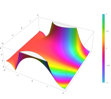
Plot of the complementary error function Erfc(z) in the complex plane from -2-2i to 2+2i with colors created with Mathematica 13.1 function ComplexPlot3D

${\begin{aligned}\operatorname {erfc} x&=1-\operatorname {erf} x\\[5pt]&={\frac {2}{\sqrt {\pi }}}\int _{x}^{\infty }e^{-t^{2}}\,\mathrm {d} t\\[5pt]&=e^{-x^{2}}\operatorname {erfcx} x,\end{aligned}}$

이는 역시 스케일된 여 오차 함수(scaled complementary error function) erfcx를 정의합니다 (이는 산술 언더플로(arithmetic underflow)를 방지하기 위해 erfc 대신 사용될 수 있습니다). x ≥ 0에 대해 erfc x의 또 다른 형식은 발견자의 이름을 따서 크레이그의 공식(Craig's formula)으로 알려져 있습니다:

$\operatorname {erfc} (x\mid x\geq 0)={\frac {2}{\pi }}\int _{0}^{\frac {\pi }{2}}\exp \left(-{\frac {x^{2}}{\sin ^{2}\theta }}\right)\,\mathrm {d} \theta .$

이 표현은 x의 양수 값에 대해서만 유효하지만, 그것은 음수 값에 대한 erfc(x)를 얻기 위해 erfc x = 2 − erfc(−x)와 결합에서 사용될 수 있습니다. 이 형식은 적분의 범위가 고정되고 유한하다는 점에서 유리합니다. 두 개의 비-음의 변수의 합의 erfc에 대한 이 표현의 확장은 다음과 같습니다:

$\operatorname {erfc} (x+y\mid x,y\geq 0)={\frac {2}{\pi }}\int _{0}^{\frac {\pi }{2}}\exp \left(-{\frac {x^{2}}{\sin ^{2}\theta }}-{\frac {y^{2}}{\cos ^{2}\theta }}\right)\,\mathrm {d} \theta .$

Imaginary error function

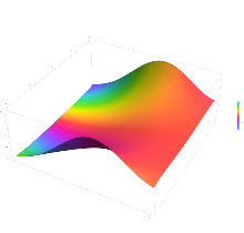
허수 오차 함수(imaginary error function)는, erfi로 표시되며, 다음으로 정의됩니다:

Plot of the imaginary error function Erfi(z) in the complex plane from -2-2i to 2+2i with colors created with Mathematica 13.1 function ComplexPlot3D

${\begin{aligned}\operatorname {erfi} x&=-i\operatorname {erf} ix\\[5pt]&={\frac {2}{\sqrt {\pi }}}\int _{0}^{x}e^{t^{2}}\,\mathrm {d} t\\[5pt]&={\frac {2}{\sqrt {\pi }}}e^{x^{2}}D(x),\end{aligned}}$

여기서 D(x)는 도슨 함수(Dawson function)입니다 (이는 산술 오버플로(arithmetic overflow)를 방지하기 위해 erfi 대신 사용할 수 있습니다).

"허수 오차 함수"라는 이름에도 불구하고, erfi x는 x가 실수일 때 실수입니다.

오차 함수가 임의적인 복소(complex) 인수 z에 대해 평가될 때, 결과 복소 오차 함수(complex error function)는 보통 파데바 함수(Faddeeva function)로 스케일된 형식에서 논의됩니다:

$w(z)=e^{-z^{2}}\operatorname {erfc} (-iz)=\operatorname {erfcx} (-iz).$

Cumulative distribution function

오차 함수는, 그것들이 스케일링과 평행이동에서만 다르기 때문에, 일부 소프트웨어 언어에 의해 norm(x)라고도 하는 Φ로 표시되는 표준 정규 누적 분포 함수(normal cumulative distribution function)와 본질적으로 동일합니다. 물론,

the normal cumulative distribution function plotted in the complex plane

${\begin{aligned}\Phi (x)&={\frac {1}{\sqrt {2\pi }}}\int _{-\infty }^{x}e^{\tfrac {-t^{2}}{2}}\,\mathrm {d} t\\[6pt]&={\frac {1}{2}}\left(1+\operatorname {erf} {\frac {x}{\sqrt {2}}}\right)\\[6pt]&={\frac {1}{2}}\operatorname {erfc} \left(-{\frac {x}{\sqrt {2}}}\right)\end{aligned}}$

또는 erf와 erfc에 대해 재정렬하여:

${\begin{aligned}\operatorname {erf} (x)&=2\Phi \left(x{\sqrt {2}}\right)-1\\[6pt]\operatorname {erfc} (x)&=2\Phi \left(-x{\sqrt {2}}\right)\\&=2\left(1-\Phi \left(x{\sqrt {2}}\right)\right).\end{aligned}}$

따라서, 오차 함수는 표준 정규 분포의 꼬리 확률인 Q-함수(Q-function)와 밀접하게 관련되어 있습니다. Q-함수는 오차 함수의 관점에서 다음과 같이 표현될 수 있습니다:

${\begin{aligned}Q(x)&={\frac {1}{2}}-{\frac {1}{2}}\operatorname {erf} {\frac {x}{\sqrt {2}}}\\&={\frac {1}{2}}\operatorname {erfc} {\frac {x}{\sqrt {2}}}.\end{aligned}}$

Φ의 역(inverse)은 정규 분위-숫자 함수(normal quantile function) 또는 프로빗(probit) 함수로 알려져 있고 역 오차 함수의 관점에서 다음과 같이 표현될 수 있습니다:

$\operatorname {probit} (p)=\Phi ^{-1}(p)={\sqrt {2}}\operatorname {erf} ^{-1}(2p-1)=-{\sqrt {2}}\operatorname {erfc} ^{-1}(2p).$

표준 정규 cdf는 확률과 통계에서 더 자주 사용되고, 오차 함수는 다른 수학 가지에서 더 자주 사용됩니다.

오차 함수는 미타그–레플레르 함수(Mittag-Leffler function)의 특수한 경우이고, 합류 초기하 함수(confluent hypergeometric function, 쿠머(Kummer)의 함수)로 표현할 수도 있습니다:

$\operatorname {erf} x={\frac {2x}{\sqrt {\pi }}}M\left({\tfrac {1}{2}},{\tfrac {3}{2}},-x^{2}\right).$

그것은 프레넬 적분(Fresnel integral)의 관점에서 간단한 표현을 가지고 있습니다.

조절된 감마 함수(regularized gamma function) P와 불완전 감마 함수(incomplete gamma function)의 관점에서,

$\operatorname {erf} x=\operatorname {sgn} x\cdot P\left({\tfrac {1}{2}},x^{2}\right)={\frac {\operatorname {sgn} x}{\sqrt {\pi }}}\gamma \left({\tfrac {1}{2}},x^{2}\right).$

여기서 sgn x는 부호 함수(sign function)입니다.

Generalized error functions

Graph of generalised error functions E_n(x):
grey curve: E₁(x) = 1 − e^−x/√π
red curve: E₂(x) = erf(x)
green curve: E₃(x)
blue curve: E₄(x)
gold curve: E₅(x).

일부 저자는 보다 일반적인 함수에 대해 논의합니다:

$E_{n}(x)={\frac {n!}{\sqrt {\pi }}}\int _{0}^{x}e^{-t^{n}}\,\mathrm {d} t={\frac {n!}{\sqrt {\pi }}}\sum _{p=0}^{\infty }(-1)^{p}{\frac {x^{np+1}}{(np+1)p!}}.$

주목할만한 사례는 다음과 같습니다:

• E₀(x)는 원점을 지나는 직선입니다: E₀(x) = x/e√π
• E₂(x)는 오차 함수입니다, erf x.

n!으로 나눈 후, 홀수 n에 대한 모든 E_n은 서로 비슷해 보입니다 (그러나 동일하지는 않습니다). 유사하게, 짝수 n에 대해 E_n은 n!에 의한 간단한 나눗셈 후에 서로 비슷해 보입니다 (그러나 동일하지는 않습니다). n > 0에 대해 모든 일반화된 오차 함수는 그래프의 양수 x 측에서 비슷하게 보입니다.

이들 일반화된 함수는 감마 함수(gamma function)와 불완전 감마 함수(incomplete gamma function)를 사용하여 x > 0에 대해 동등하게 표현될 수 있습니다:

$E_{n}(x)={\frac {1}{\sqrt {\pi }}}\Gamma (n)\left(\Gamma \left({\frac {1}{n}}\right)-\Gamma \left({\frac {1}{n}},x^{n}\right)\right),\qquad x>0.$

그러므로, 우리는 불완전 감마 함수의 관점에서 오차 함수를 정의할 수 있습니다:

$\operatorname {erf} x=1-{\frac {1}{\sqrt {\pi }}}\Gamma \left({\tfrac {1}{2}},x^{2}\right).$

Iterated integrals of the complementary error function

여 오차 함수의 반복된 적분은 다음에 의해 정의됩니다

${\begin{aligned}\operatorname {i} ^{n}\!\operatorname {erfc} z&=\int _{z}^{\infty }\operatorname {i} ^{n-1}\!\operatorname {erfc} \zeta \,\mathrm {d} \zeta \\[6pt]\operatorname {i} ^{0}\!\operatorname {erfc} z&=\operatorname {erfc} z\\\operatorname {i} ^{1}\!\operatorname {erfc} z&=\operatorname {ierfc} z={\frac {1}{\sqrt {\pi }}}e^{-z^{2}}-z\operatorname {erfc} z\\\operatorname {i} ^{2}\!\operatorname {erfc} z&={\tfrac {1}{4}}\left(\operatorname {erfc} z-2z\operatorname {ierfc} z\right)\\\end{aligned}}$

일반적인 재귀 공식은 다음과 같습니다:

$2n\cdot \operatorname {i} ^{n}\!\operatorname {erfc} z=\operatorname {i} ^{n-2}\!\operatorname {erfc} z-2z\cdot \operatorname {i} ^{n-1}\!\operatorname {erfc} z$

그것들은 다음 거듭제곱 급수를 가집니다:

$\operatorname {i} ^{n}\!\operatorname {erfc} z=\sum _{j=0}^{\infty }{\frac {(-z)^{j}}{2^{n-j}j!\,\Gamma \left(1+{\frac {n-j}{2}}\right)}},$

이로부터 다음 대칭 속성임이 따릅니다:

$\operatorname {i} ^{2m}\!\operatorname {erfc} (-z)=-\operatorname {i} ^{2m}\!\operatorname {erfc} z+\sum _{q=0}^{m}{\frac {z^{2q}}{2^{2(m-q)-1}(2q)!(m-q)!}}$

및

$\operatorname {i} ^{2m+1}\!\operatorname {erfc} (-z)=\operatorname {i} ^{2m+1}\!\operatorname {erfc} z+\sum _{q=0}^{m}{\frac {z^{2q+1}}{2^{2(m-q)-1}(2q+1)!(m-q)!}}.$

Implementations

As real function of a real argument

• Posix-호환 운영 시스템에서, 헤더 math.h는 선언되어야 하고 수학 라이브러리 libm은 함수 erf 및 erfc (두배 정밀도(double precision)) 와 단일 정밀도(single precision)와 확장된 정밀도(extended precision) 짝 erff, erfl 및 erfcf, erfcl을 제공합니다.
• GNU Scientific Library는 erf, erfc, log(erf), 및 스케일된 오차 함수를 제공합니다.

As complex function of a complex argument

• libcerf, 복소 오차 함수에 대해 숫자 C 라이브러리는 MIT Faddeeva Package에 구현된 파데바 함수를 기반으로 복소 함수 cerf, cerfc, cerfcx 및 실수 함수 erfi, erfcx를 근사적으로 13–14 자리 정밀도로 제공합니다.

See also

Related functions

• Gaussian integral, over the whole real line
• Gaussian function, derivative
• Dawson function, renormalized imaginary error function
• Goodwin–Staton integral

In probability

• Normal distribution
• Normal cumulative distribution function, a scaled and shifted form of error function
• Probit, the inverse or quantile function of the normal CDF
• Q-function, the tail probability of the normal distribution

Further reading

• Abramowitz, Milton; Stegun, Irene Ann, eds. (1983) [June 1964]. "Chapter 7". Handbook of Mathematical Functions with Formulas, Graphs, and Mathematical Tables. Applied Mathematics Series. Vol. 55 (Ninth reprint with additional corrections of tenth original printing with corrections (December 1972); first ed.). Washington D.C.; New York: United States Department of Commerce, National Bureau of Standards; Dover Publications. p. 297. ISBN 978-0-486-61272-0. LCCN 64-60036. MR 0167642. LCCN 65-12253.
• Press, William H.; Teukolsky, Saul A.; Vetterling, William T.; Flannery, Brian P. (2007), "Section 6.2. Incomplete Gamma Function and Error Function", Numerical Recipes: The Art of Scientific Computing (3rd ed.), New York: Cambridge University Press, ISBN 978-0-521-88068-8
• Temme, Nico M. (2010), "Error Functions, Dawson's and Fresnel Integrals", in Olver, Frank W. J.; Lozier, Daniel M.; Boisvert, Ronald F.; Clark, Charles W. (eds.), NIST Handbook of Mathematical Functions, Cambridge University Press, ISBN 978-0521192255, MR 2723248

External links

• A Table of Integrals of the Error Functions

References

- ^ Andrews, Larry C. (1998). Special functions of mathematics for engineers. SPIE Press. p. 110. ISBN 9780819426161.
- ^ Glaisher, James Whitbread Lee (July 1871). "On a class of definite integrals". London, Edinburgh, and Dublin Philosophical Magazine and Journal of Science. 4. 42 (277): 294–302. doi:10.1080/14786447108640568. Retrieved 6 December 2017.
- ^ Glaisher, James Whitbread Lee (September 1871). "On a class of definite integrals. Part II". London, Edinburgh, and Dublin Philosophical Magazine and Journal of Science. 4. 42 (279): 421–436. doi:10.1080/14786447108640600. Retrieved 6 December 2017.
- ^ "A007680 – OEIS". oeis.org. Retrieved 2020-04-02.
- ^ Weisstein, Eric W. "Erf". MathWorld.
- ^ Schöpf, H. M.; Supancic, P. H. (2014). "On Bürmann's Theorem and Its Application to Problems of Linear and Nonlinear Heat Transfer and Diffusion". The Mathematica Journal. 16. doi:10.3888/tmj.16-11.
- ^ Weisstein, Eric W. "Bürmann's Theorem". MathWorld.
- ^ Bergsma, Wicher (2006). "On a new correlation coefficient, its orthogonal decomposition and associated tests of independence". arXiv:math/0604627.
- ^ Cuyt, Annie A. M.; Petersen, Vigdis B.; Verdonk, Brigitte; Waadeland, Haakon; Jones, William B. (2008). Handbook of Continued Fractions for Special Functions. Springer-Verlag. ISBN 978-1-4020-6948-2.
- ^ Ng, Edward W.; Geller, Murray (January 1969). "A table of integrals of the Error functions". Journal of Research of the National Bureau of Standards Section B. 73B (1): 1. doi:10.6028/jres.073B.001.
- ^ Schlömilch, Oskar Xavier (1859). "Ueber facultätenreihen". Zeitschrift für Mathematik und Physik (in German). 4: 390–415. Retrieved 2017-12-04.
- ^ Nielson, Niels (1906). Handbuch der Theorie der Gammafunktion (in German). Leipzig: B. G. Teubner. p. 283 Eq. 3. Retrieved 2017-12-04.
- ^ Chiani, M.; Dardari, D.; Simon, M.K. (2003). "New Exponential Bounds and Approximations for the Computation of Error Probability in Fading Channels" (PDF). IEEE Transactions on Wireless Communications. 2 (4): 840–845. CiteSeerX 10.1.1.190.6761. doi:10.1109/TWC.2003.814350.
- ^ Tanash, I.M.; Riihonen, T. (2020). "Global minimax approximations and bounds for the Gaussian Q-function by sums of exponentials". IEEE Transactions on Communications. 68 (10): 6514–6524. arXiv:2007.06939. doi:10.1109/TCOMM.2020.3006902. S2CID 220514754.
- ^ Tanash, I.M.; Riihonen, T. (2020). "Coefficients for Global Minimax Approximations and Bounds for the Gaussian Q-Function by Sums of Exponentials [Data set]". Zenodo. doi:10.5281/zenodo.4112978.
- ^ Karagiannidis, G. K.; Lioumpas, A. S. (2007). "An improved approximation for the Gaussian Q-function" (PDF). IEEE Communications Letters. 11 (8): 644–646. doi:10.1109/LCOMM.2007.070470. S2CID 4043576.
- ^ Tanash, I.M.; Riihonen, T. (2021). "Improved coefficients for the Karagiannidis–Lioumpas approximations and bounds to the Gaussian Q-function". IEEE Communications Letters. 25 (5): 1468–1471. arXiv:2101.07631. doi:10.1109/LCOMM.2021.3052257. S2CID 231639206.
- ^ Chang, Seok-Ho; Cosman, Pamela C.; Milstein, Laurence B. (November 2011). "Chernoff-Type Bounds for the Gaussian Error Function". IEEE Transactions on Communications. 59 (11): 2939–2944. doi:10.1109/TCOMM.2011.072011.100049. S2CID 13636638.
- ^ Winitzki, Sergei (2003). "Uniform approximations for transcendental functions". Computational Science and Its Applications – ICCSA 2003. Lecture Notes in Computer Science. Vol. 2667. Springer, Berlin. pp. 780–789. doi:10.1007/3-540-44839-X_82. ISBN 978-3-540-40155-1.
- ^ Zeng, Caibin; Chen, Yang Cuan (2015). "Global Padé approximations of the generalized Mittag-Leffler function and its inverse". Fractional Calculus and Applied Analysis. 18 (6): 1492–1506. arXiv:1310.5592. doi:10.1515/fca-2015-0086. S2CID 118148950.
Indeed, Winitzki [32] provided the so-called global Padé approximation
- ^ Winitzki, Sergei (6 February 2008). "A handy approximation for the error function and its inverse".
{{cite journal}}: Cite journal requires|journal=(help) - ^ Numerical Recipes in Fortran 77: The Art of Scientific Computing (ISBN 0-521-43064-X), 1992, page 214, Cambridge University Press.
- ^ a b c Cody, W. J. (March 1993), "Algorithm 715: SPECFUN—A portable FORTRAN package of special function routines and test drivers" (PDF), ACM Trans. Math. Softw., 19 (1): 22–32, CiteSeerX 10.1.1.643.4394, doi:10.1145/151271.151273, S2CID 5621105
- ^ Zaghloul, M. R. (1 March 2007), "On the calculation of the Voigt line profile: a single proper integral with a damped sine integrand", Monthly Notices of the Royal Astronomical Society, 375 (3): 1043–1048, Bibcode:2007MNRAS.375.1043Z, doi:10.1111/j.1365-2966.2006.11377.x
- ^ John W. Craig, A new, simple and exact result for calculating the probability of error for two-dimensional signal constellations Archived 3 April 2012 at the Wayback Machine, Proceedings of the 1991 IEEE Military Communication Conference, vol. 2, pp. 571–575.
- ^ Behnad, Aydin (2020). "A Novel Extension to Craig's Q-Function Formula and Its Application in Dual-Branch EGC Performance Analysis". IEEE Transactions on Communications. 68 (7): 4117–4125. doi:10.1109/TCOMM.2020.2986209. S2CID 216500014.
- ^ Carslaw, H. S.; Jaeger, J. C. (1959), Conduction of Heat in Solids (2nd ed.), Oxford University Press, ISBN 978-0-19-853368-9, p 484
- ^ https://pubs.opengroup.org/onlinepubs/9699919799/basedefs/math.h.html
- ^ "Special Functions – GSL 2.7 documentation".